大模型、深度学习、人工智能……这些词我们经常听到,但它们背后的核心是什么?答案是:神经网络 。神经网络是现代 AI 的基础。从手机上的语音助手,到 AlphaGo 战胜围棋世界冠军,再到 ChatGPT 能写诗、编程、回答问题,背后都是神经网络在"思考"。那么,神经网络到底是什么?它是如何"学习"的?这篇文章将用一个生活中的例子——预测孩子身高 ,带你从零开始理解神经网络的核心概念:
神经网络 :一个由简单计算单元组成的"大脑"梯度 :告诉模型"该往哪个方向调整"的信号反向传播 :高效计算梯度的巧妙算法
不需要任何数学基础,让我们开始吧。
从身高预测开始
假设你想预测你未来孩子的身高。一个简单的想法是:孩子的身高和父母身高有关。于是你写出一个公式:
孩子身高 = w 1 × 父亲身高 + w 2 × 母亲身高 \text{孩子身高} = w_1 \times \text{父亲身高} + w_2 \times \text{母亲身高}
孩子身高 = w 1 × 父亲身高 + w 2 × 母亲身高
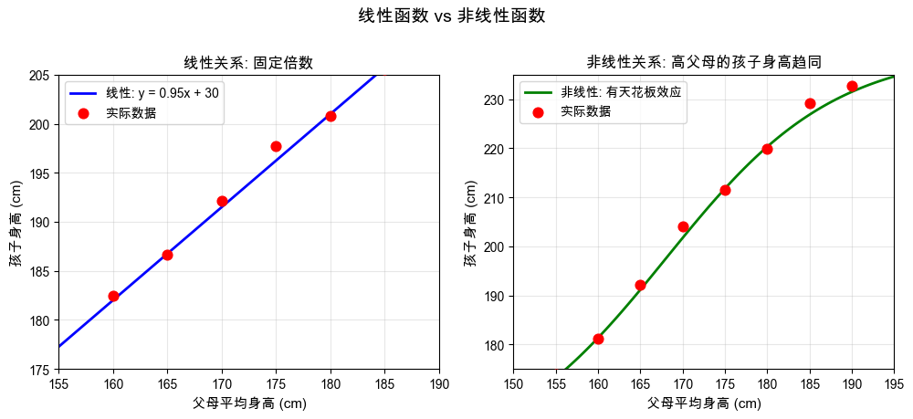
这个公式就是一个线性函数 。直觉上可以认为孩子的身高一半继承父亲,一半继承母亲,所以可以设 w 1 = 0.5 w_1 = 0.5 w 1 = 0.5 w 2 = 0.5 w_2 = 0.5 w 2 = 0.5 0.5 × 178 + 0.5 × 165 = 171.5 0.5 \times 178 + 0.5 \times 165 = 171.5 0.5 × 178 + 0.5 × 165 = 171.5
这个简单的公式可以认为是一个模型,具体来说,这是一个单层神经网络 。父亲身高、母亲身高是输入,孩子身高是输出,w 1 w_1 w 1 w 2 w_2 w 2 参数 (也叫权重)。
线性不够,激活来凑
但你很快发现,实际情况没这么简单。父母身高高,孩子大概率高,但不是简单的线性倍数关系。身高的预测存在一个非线性 的关系,使得下一代的身高回归平均水平,比如会一个"天花板"效应——父母都超高时,孩子不一定比父母更高。
于是我们需要引入激活函数 ,把线性计算的结果做一下非线性变换:
预测身高 = f ( w 1 × 父亲身高 + w 2 × 母亲身高 ) \text{预测身高} = f(w_1 \times \text{父亲身高} + w_2 \times \text{母亲身高})
预测身高 = f ( w 1 × 父亲身高 + w 2 × 母亲身高 )
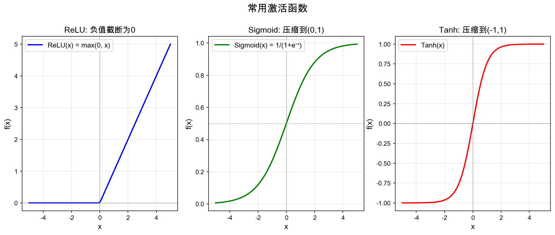
这里的f f f f ( x ) = tanh ( x ) f(x) = \tanh(x) f ( x ) = tanh ( x ) f ( x ) = max ( 0 , x ) f(x) = \max(0, x) f ( x ) = max ( 0 , x ) f ( x ) = 1 1 + e − x f(x) = \frac{1}{1+e^{-x}} f ( x ) = 1 + e − x 1 深入了解可参考这里 。
更多因素:多层网络
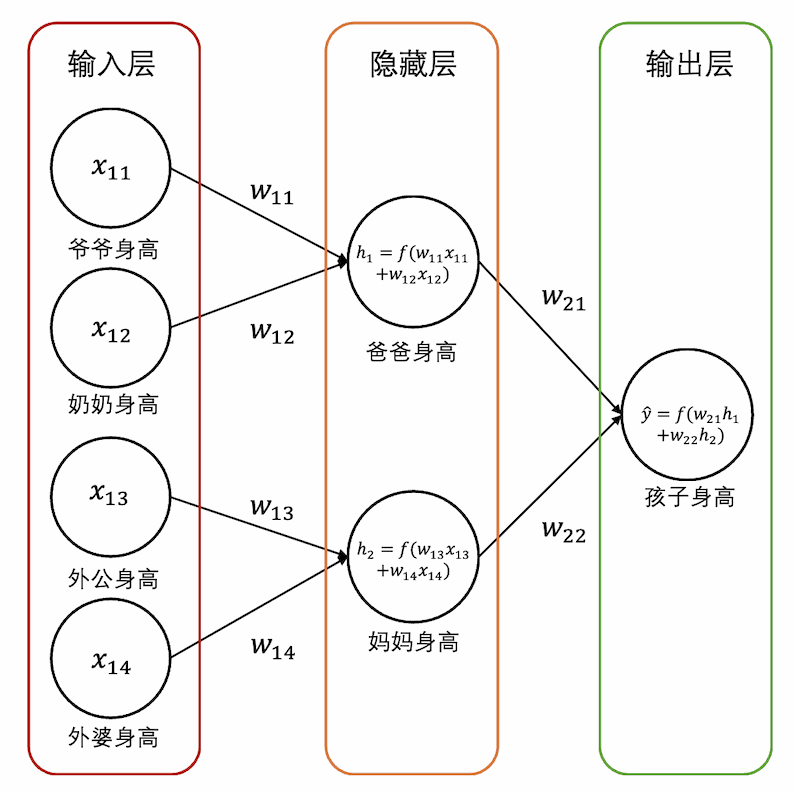
现实中的身高预测还要考虑更多因素。比如孩子的身高还和祖父母的身高 有关。于是模型变得更复杂:
第一层 :从祖父母身高预测父母身高
父亲身高 = f ( w 11 × 爷爷身高 + w 12 × 奶奶身高 ) \text{父亲身高} = f(w_{11} \times \text{爷爷身高} + w_{12} \times \text{奶奶身高})
父亲身高 = f ( w 11 × 爷爷身高 + w 12 × 奶奶身高 )
母亲身高 = f ( w 13 × 外公身高 + w 14 × 外婆身高 ) \text{母亲身高} = f(w_{13} \times \text{外公身高} + w_{14} \times \text{外婆身高})
母亲身高 = f ( w 13 × 外公身高 + w 14 × 外婆身高 )
第二层 :从父母身高预测孩子身高
孩子身高 = f ( w 21 × 父亲身高 + w 22 × 母亲身高 ) \text{孩子身高} = f(w_{21} \times \text{父亲身高} + w_{22} \times \text{母亲身高})
孩子身高 = f ( w 21 × 父亲身高 + w 22 × 母亲身高 )
这就是一个两层神经网络 。每一层都有自己的参数,一层的输出作为下一层的输入。
更一般地,一个 L L L
h 1 = f ( W 1 x ) h_1 = f(W_1 x)
h 1 = f ( W 1 x )
h 2 = f ( W 2 h 1 ) h_2 = f(W_2 h_1)
h 2 = f ( W 2 h 1 )
⋮ \vdots
⋮
y ^ = f ( W L h L − 1 ) \hat{y} = f(W_L h_{L-1})
y ^ = f ( W L h L − 1 )
其中 x x x y ^ \hat{y} y ^ W 1 , W 2 , … , W L W_1, W_2, \ldots, W_L W 1 , W 2 , … , W L
如何调整参数:梯度下降
上面的网络有很多参数(w 1 , w 2 , W 1 , W 2 , … w_1, w_2, W_1, W_2, \ldots w 1 , w 2 , W 1 , W 2 , …
核心思想 :用已有数据来训练。比如你收集了1000个家庭的祖父母、父母、孩子身高数据。对每个家庭,计算预测值y ^ \hat{y} y ^ y y y
L = 1 2 ( y ^ − y ) 2 \mathcal{L} = \frac{1}{2}(\hat{y} - y)^2
L = 2 1 ( y ^ − y ) 2
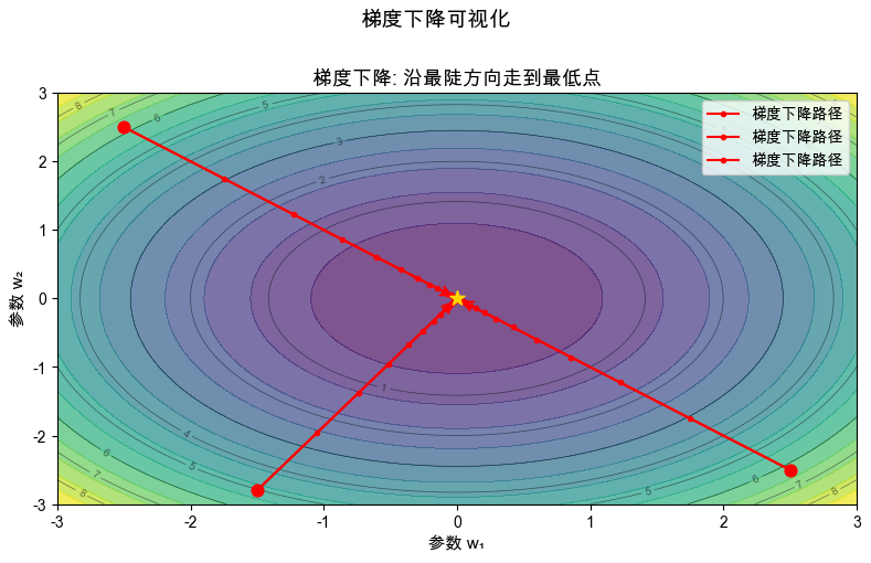
然后想办法调整参数,让损失尽量小。那要怎么调整每个参数呢?直觉上,如果预测出来的值比真实值高,那么可以修改假设,认为孩子的身高不是继承一半父亲的身高,可以适当地减小w 1 w_1 w 1 梯度 。让参数沿着梯度,也就是使损失下降最快的方向调 。具体来说,对每个参数 w i w_i w i ∂ L ∂ w i \frac{\partial \mathcal{L}}{\partial w_i} ∂ w i ∂ L
w i ← w i − η ⋅ ∂ L ∂ w i w_i \leftarrow w_i - \eta \cdot \frac{\partial \mathcal{L}}{\partial w_i}
w i ← w i − η ⋅ ∂ w i ∂ L
其中 η \eta η 梯度下降 。
梯度是什么
梯度 就是损失函数对每个参数的偏导数。它告诉你:如果稍微增加一点参数 w i w_i w i
举个直观的例子:你在山上,想最快下山。你看看四周哪个方向最陡(导数最大),就往那个方向走一步。梯度就是告诉你"哪个方向最陡"的那个量。
对于身高预测的例子,如果 ∂ L ∂ w 1 = 5 \frac{\partial \mathcal{L}}{\partial w_1} = 5 ∂ w 1 ∂ L = 5 w 1 w_1 w 1 w 1 w_1 w 1 ∂ L ∂ w 1 = − 3 \frac{\partial \mathcal{L}}{\partial w_1} = -3 ∂ w 1 ∂ L = − 3 w 1 w_1 w 1 w 1 w_1 w 1 w 1 w_1 w 1
反向传播:高效计算梯度
在多层网络中,参数可能有成千上万个。如果对每个参数都单独算导数,计算量会非常大。反向传播 利用链式法则 ,从输出层开始,逐层往回算梯度。这是深度学习高效训练的关键。
6.1 用身高例子说明
假设我们有:
a = 父亲身高 = 178 a = \text{父亲身高} = 178
a = 父亲身高 = 178
b = 母亲身高 = 165 b = \text{母亲身高} = 165
b = 母亲身高 = 165
c = w 1 a + w 2 b c = w_1 a + w_2 b
c = w 1 a + w 2 b
y ^ = f ( c ) \hat{y} = f(c)
y ^ = f ( c )
L = 1 2 ( y ^ − y ) 2 \mathcal{L} = \frac{1}{2}(\hat{y} - y)^2
L = 2 1 ( y ^ − y ) 2
设 w 1 = 0.5 w_1 = 0.5 w 1 = 0.5 w 2 = 0.5 w_2 = 0.5 w 2 = 0.5 y = 175 y = 175 y = 175 f ( x ) = x f(x) = x f ( x ) = x
前向传播 :
c = 0.5 × 178 + 0.5 × 165 = 171.5 c = 0.5 \times 178 + 0.5 \times 165 = 171.5 c = 0.5 × 178 + 0.5 × 165 = 171.5 y ^ = 171.5 \hat{y} = 171.5 y ^ = 171.5 L = 1 2 ( 171.5 − 175 ) 2 = 7.225 \mathcal{L} = \frac{1}{2}(171.5 - 175)^2 = 7.225 L = 2 1 ( 171.5 − 175 ) 2 = 7.225
反向传播 (从后往前算):
损失对预测值的梯度:
∂ L ∂ y ^ = y ^ − y = 171.5 − 175 = − 3.5 \frac{\partial \mathcal{L}}{\partial \hat{y}} = \hat{y} - y = 171.5 - 175 = -3.5
∂ y ^ ∂ L = y ^ − y = 171.5 − 175 = − 3.5
预测值对 c c c f f f
∂ y ^ ∂ c = 1 \frac{\partial \hat{y}}{\partial c} = 1
∂ c ∂ y ^ = 1
由链式法则,损失对 c c c
∂ L ∂ c = ∂ L ∂ y ^ ⋅ ∂ y ^ ∂ c = − 3.5 × 1 = − 3.5 \frac{\partial \mathcal{L}}{\partial c} = \frac{\partial \mathcal{L}}{\partial \hat{y}} \cdot \frac{\partial \hat{y}}{\partial c} = -3.5 \times 1 = -3.5
∂ c ∂ L = ∂ y ^ ∂ L ⋅ ∂ c ∂ y ^ = − 3.5 × 1 = − 3.5
c c c w 1 w_1 w 1
∂ c ∂ w 1 = a = 178 \frac{\partial c}{\partial w_1} = a = 178
∂ w 1 ∂ c = a = 178
由链式法则,损失对 w 1 w_1 w 1
∂ L ∂ w 1 = ∂ L ∂ c ⋅ ∂ c ∂ w 1 = − 3.5 × 178 = − 623 \frac{\partial \mathcal{L}}{\partial w_1} = \frac{\partial \mathcal{L}}{\partial c} \cdot \frac{\partial c}{\partial w_1} = -3.5 \times 178 = -623
∂ w 1 ∂ L = ∂ c ∂ L ⋅ ∂ w 1 ∂ c = − 3.5 × 178 = − 623
类似地,损失对 w 2 w_2 w 2
∂ L ∂ w 2 = − 3.5 × 165 = − 577.5 \frac{\partial \mathcal{L}}{\partial w_2} = -3.5 \times 165 = -577.5
∂ w 2 ∂ L = − 3.5 × 165 = − 577.5
更新参数 (设学习率 η = 0.001 \eta = 0.001 η = 0.001
w 1 ← 0.5 − 0.001 × ( − 623 ) = 0.5623 w_1 \leftarrow 0.5 - 0.001 \times (-623) = 0.5623 w 1 ← 0.5 − 0.001 × ( − 623 ) = 0.5623 w 2 ← 0.5 − 0.001 × ( − 577.5 ) = 0.5578 w_2 \leftarrow 0.5 - 0.001 \times (-577.5) = 0.5578 w 2 ← 0.5 − 0.001 × ( − 577.5 ) = 0.5578
可以看到,w 1 w_1 w 1 w 2 w_2 w 2
各种运算的梯度
在实际神经网络中,会用到加、减、乘、除、激活函数等各种运算。下面逐一介绍它们的梯度计算和传播方式。
加法 c = a + b c = a + b c = a + b
前向 :c = a + b c = a + b c = a + b
反向 :∂ c ∂ a = 1 \frac{\partial c}{\partial a} = 1 ∂ a ∂ c = 1 ∂ c ∂ b = 1 \frac{\partial c}{\partial b} = 1 ∂ b ∂ c = 1
梯度直接传递给两个输入:
∂ L ∂ a = ∂ L ∂ c × 1 = ∂ L ∂ c \frac{\partial \mathcal{L}}{\partial a} = \frac{\partial \mathcal{L}}{\partial c} \times 1 = \frac{\partial \mathcal{L}}{\partial c} ∂ a ∂ L = ∂ c ∂ L × 1 = ∂ c ∂ L ∂ L ∂ b = ∂ L ∂ c × 1 = ∂ L ∂ c \frac{\partial \mathcal{L}}{\partial b} = \frac{\partial \mathcal{L}}{\partial c} \times 1 = \frac{\partial \mathcal{L}}{\partial c} ∂ b ∂ L = ∂ c ∂ L × 1 = ∂ c ∂ L
特点 :上层梯度直接复制到两个输入。
乘法 c = a × b c = a \times b c = a × b
前向 :c = a × b c = a \times b c = a × b
反向 :∂ c ∂ a = b \frac{\partial c}{\partial a} = b ∂ a ∂ c = b ∂ c ∂ b = a \frac{\partial c}{\partial b} = a ∂ b ∂ c = a
梯度传递:∂ L ∂ a = ∂ L ∂ c × b \frac{\partial \mathcal{L}}{\partial a} = \frac{\partial \mathcal{L}}{\partial c} \times b ∂ a ∂ L = ∂ c ∂ L × b ∂ L ∂ b = ∂ L ∂ c × a \frac{\partial \mathcal{L}}{\partial b} = \frac{\partial \mathcal{L}}{\partial c} \times a ∂ b ∂ L = ∂ c ∂ L × a
特点 :乘法的梯度传递依赖另一个输入的值。
幂运算 c = a b c = a^b c = a b
前向 :c = a b c = a^b c = a b
反向 :∂ c ∂ a = b ⋅ a b − 1 \frac{\partial c}{\partial a} = b \cdot a^{b-1} ∂ a ∂ c = b ⋅ a b − 1 ∂ c ∂ b = a b ⋅ ln ( a ) \frac{\partial c}{\partial b} = a^b \cdot \ln(a) ∂ b ∂ c = a b ⋅ ln ( a )
梯度传递:∂ L ∂ a = ∂ L ∂ c × b ⋅ a b − 1 \frac{\partial \mathcal{L}}{\partial a} = \frac{\partial \mathcal{L}}{\partial c} \times b \cdot a^{b-1} ∂ a ∂ L = ∂ c ∂ L × b ⋅ a b − 1 ∂ L ∂ b = ∂ L ∂ c × a b ⋅ ln ( a ) \frac{\partial \mathcal{L}}{\partial b} = \frac{\partial \mathcal{L}}{\partial c} \times a^b \cdot \ln(a) ∂ b ∂ L = ∂ c ∂ L × a b ⋅ ln ( a )
常用特例 :c = a 2 c = a^2 c = a 2 ∂ L ∂ a = ∂ L ∂ c × 2 a \frac{\partial \mathcal{L}}{\partial a} = \frac{\partial \mathcal{L}}{\partial c} \times 2a ∂ a ∂ L = ∂ c ∂ L × 2 a
除法 c = a b c = \frac{a}{b} c = b a
前向 :c = a b c = \frac{a}{b} c = b a
反向 :∂ c ∂ a = 1 b \frac{\partial c}{\partial a} = \frac{1}{b} ∂ a ∂ c = b 1 ∂ c ∂ b = − a b 2 \frac{\partial c}{\partial b} = -\frac{a}{b^2} ∂ b ∂ c = − b 2 a
梯度传递:∂ L ∂ a = ∂ L ∂ c × 1 b \frac{\partial \mathcal{L}}{\partial a} = \frac{\partial \mathcal{L}}{\partial c} \times \frac{1}{b} ∂ a ∂ L = ∂ c ∂ L × b 1 ∂ L ∂ b = ∂ L ∂ c × ( − a b 2 ) \frac{\partial \mathcal{L}}{\partial b} = \frac{\partial \mathcal{L}}{\partial c} \times (-\frac{a}{b^2}) ∂ b ∂ L = ∂ c ∂ L × ( − b 2 a )
注意 :除法对分母的梯度是负的,且当 b b b
激活函数
ReLU:f ( x ) = max ( 0 , x ) f(x) = \max(0, x) f ( x ) = max ( 0 , x )
前向 :y = max ( 0 , x ) y = \max(0, x) y = max ( 0 , x )
反向 :d y d x = { 1 if x > 0 0 if x ≤ 0 \frac{dy}{dx} = \begin{cases} 1 & \text{if } x > 0 \\ 0 & \text{if } x \leq 0 \end{cases} d x d y = { 1 0 if x > 0 if x ≤ 0
梯度传递:∂ L ∂ x = ∂ L ∂ y × { 1 if x > 0 0 if x ≤ 0 \frac{\partial \mathcal{L}}{\partial x} = \frac{\partial \mathcal{L}}{\partial y} \times \begin{cases} 1 & \text{if } x > 0 \\ 0 & \text{if } x \leq 0 \end{cases} ∂ x ∂ L = ∂ y ∂ L × { 1 0 if x > 0 if x ≤ 0
特点 :正区间梯度=1,直接传递;负区间梯度=0,被截断。
Sigmoid:f ( x ) = 1 1 + e − x f(x) = \frac{1}{1+e^{-x}} f ( x ) = 1 + e − x 1
前向 :y = 1 1 + e − x y = \frac{1}{1+e^{-x}} y = 1 + e − x 1
反向 :d y d x = y ( 1 − y ) \frac{dy}{dx} = y(1-y) d x d y = y ( 1 − y )
梯度传递:∂ L ∂ x = ∂ L ∂ y × y ( 1 − y ) \frac{\partial \mathcal{L}}{\partial x} = \frac{\partial \mathcal{L}}{\partial y} \times y(1-y) ∂ x ∂ L = ∂ y ∂ L × y ( 1 − y )
特点 :导数最大值为0.25,在饱和区(∣ x ∣ |x| ∣ x ∣
Tanh:f ( x ) = tanh ( x ) f(x) = \tanh(x) f ( x ) = tanh ( x )
前向 :y = tanh ( x ) y = \tanh(x) y = tanh ( x )
反向 :d y d x = 1 − y 2 \frac{dy}{dx} = 1 - y^2 d x d y = 1 − y 2
梯度传递:∂ L ∂ x = ∂ L ∂ y × ( 1 − y 2 ) \frac{\partial \mathcal{L}}{\partial x} = \frac{\partial \mathcal{L}}{\partial y} \times (1 - y^2) ∂ x ∂ L = ∂ y ∂ L × ( 1 − y 2 )
求和 c = ∑ i a i c = \sum_i a_i c = ∑ i a i
前向 :c = a 1 + a 2 + ⋯ + a n c = a_1 + a_2 + \cdots + a_n c = a 1 + a 2 + ⋯ + a n
反向 :∂ c ∂ a i = 1 \frac{\partial c}{\partial a_i} = 1 ∂ a i ∂ c = 1 i i i
梯度传递:每个输入得到相同的梯度。
取负 c = − a c = -a c = − a
前向 :c = − a c = -a c = − a
反向 :∂ c ∂ a = − 1 \frac{\partial c}{\partial a} = -1 ∂ a ∂ c = − 1
梯度传递:∂ L ∂ a = − ∂ L ∂ c \frac{\partial \mathcal{L}}{\partial a} = -\frac{\partial \mathcal{L}}{\partial c} ∂ a ∂ L = − ∂ c ∂ L
完整示例:一个小型神经网络
让我们用一个具体的例子,把上面的知识串起来。
网络结构 :
输入:x 1 = 2 x_1 = 2 x 1 = 2 x 2 = 3 x_2 = 3 x 2 = 3
第一层:h 1 = w 1 x 1 + w 2 x 2 h_1 = w_1 x_1 + w_2 x_2 h 1 = w 1 x 1 + w 2 x 2 h 2 = w 3 x 1 + w 4 x 2 h_2 = w_3 x_1 + w_4 x_2 h 2 = w 3 x 1 + w 4 x 2
激活:a 1 = ReLU ( h 1 ) a_1 = \text{ReLU}(h_1) a 1 = ReLU ( h 1 ) a 2 = ReLU ( h 2 ) a_2 = \text{ReLU}(h_2) a 2 = ReLU ( h 2 )
输出:y ^ = w 5 a 1 + w 6 a 2 \hat{y} = w_5 a_1 + w_6 a_2 y ^ = w 5 a 1 + w 6 a 2
损失:L = 1 2 ( y ^ − y ) 2 \mathcal{L} = \frac{1}{2}(\hat{y} - y)^2 L = 2 1 ( y ^ − y ) 2 y = 10 y = 10 y = 10
参数初始化 :w 1 = 1 , w 2 = 1 , w 3 = 1 , w 4 = 1 , w 5 = 1 , w 6 = 1 w_1=1, w_2=1, w_3=1, w_4=1, w_5=1, w_6=1 w 1 = 1 , w 2 = 1 , w 3 = 1 , w 4 = 1 , w 5 = 1 , w 6 = 1
前向传播
1
2
3
4
5
6
h_1 = w_1 x_1 + w_2 x_2 = 1×2 + 1×3 = 5 h_2 = w_3 x_1 + w_4 x_2 = 1×2 + 1×3 = 5 a_1 = ReLU(h_1) = ReLU(5) = 5 a_2 = ReLU(h_2) = ReLU(5) = 5 ŷ = w_5 a_1 + w_6 a_2 = 1×5 + 1×5 = 10 L = ½(ŷ - y)² = ½(10 - 10)² = 0
(这个例子损失为0,说明参数已经很完美了。我们换个真实值演示。)
用一个预测不准的例子演示
设 y = 20 y = 20 y = 20
前向传播 :
h 1 = 5 h_1 = 5 h 1 = 5 h 2 = 5 h_2 = 5 h 2 = 5 a 1 = 5 a_1 = 5 a 1 = 5 a 2 = 5 a_2 = 5 a 2 = 5 y ^ = 10 \hat{y} = 10 y ^ = 10 L = 1 2 ( 10 − 20 ) 2 = 50 \mathcal{L} = \frac{1}{2}(10 - 20)^2 = 50 L = 2 1 ( 10 − 20 ) 2 = 50
反向传播 :
∂ L ∂ y ^ = y ^ − y = 10 − 20 = − 10 \frac{\partial \mathcal{L}}{\partial \hat{y}} = \hat{y} - y = 10 - 20 = -10 ∂ y ^ ∂ L = y ^ − y = 10 − 20 = − 10
∂ y ^ ∂ w 5 = a 1 = 5 \frac{\partial \hat{y}}{\partial w_5} = a_1 = 5 ∂ w 5 ∂ y ^ = a 1 = 5 ∂ y ^ ∂ a 1 = w 5 = 1 \frac{\partial \hat{y}}{\partial a_1} = w_5 = 1 ∂ a 1 ∂ y ^ = w 5 = 1
∂ L ∂ w 5 = − 10 × 5 = − 50 \frac{\partial \mathcal{L}}{\partial w_5} = -10 \times 5 = -50 ∂ w 5 ∂ L = − 10 × 5 = − 50 ∂ L ∂ a 1 = − 10 × 1 = − 10 \frac{\partial \mathcal{L}}{\partial a_1} = -10 \times 1 = -10 ∂ a 1 ∂ L = − 10 × 1 = − 10
∂ y ^ ∂ w 6 = a 2 = 5 \frac{\partial \hat{y}}{\partial w_6} = a_2 = 5 ∂ w 6 ∂ y ^ = a 2 = 5 ∂ y ^ ∂ a 2 = w 6 = 1 \frac{\partial \hat{y}}{\partial a_2} = w_6 = 1 ∂ a 2 ∂ y ^ = w 6 = 1
∂ L ∂ w 6 = − 10 × 5 = − 50 \frac{\partial \mathcal{L}}{\partial w_6} = -10 \times 5 = -50 ∂ w 6 ∂ L = − 10 × 5 = − 50 ∂ L ∂ a 2 = − 10 × 1 = − 10 \frac{\partial \mathcal{L}}{\partial a_2} = -10 \times 1 = -10 ∂ a 2 ∂ L = − 10 × 1 = − 10
ReLU反向:h 1 = 5 > 0 h_1 = 5 > 0 h 1 = 5 > 0 ∂ a 1 ∂ h 1 = 1 \frac{\partial a_1}{\partial h_1} = 1 ∂ h 1 ∂ a 1 = 1
∂ L ∂ h 1 = − 10 × 1 = − 10 \frac{\partial \mathcal{L}}{\partial h_1} = -10 \times 1 = -10 ∂ h 1 ∂ L = − 10 × 1 = − 10
ReLU反向:h 2 = 5 > 0 h_2 = 5 > 0 h 2 = 5 > 0 ∂ a 2 ∂ h 2 = 1 \frac{\partial a_2}{\partial h_2} = 1 ∂ h 2 ∂ a 2 = 1
∂ L ∂ h 2 = − 10 × 1 = − 10 \frac{\partial \mathcal{L}}{\partial h_2} = -10 \times 1 = -10 ∂ h 2 ∂ L = − 10 × 1 = − 10
∂ h 1 ∂ w 1 = x 1 = 2 \frac{\partial h_1}{\partial w_1} = x_1 = 2 ∂ w 1 ∂ h 1 = x 1 = 2 ∂ h 1 ∂ w 2 = x 2 = 3 \frac{\partial h_1}{\partial w_2} = x_2 = 3 ∂ w 2 ∂ h 1 = x 2 = 3
∂ L ∂ w 1 = − 10 × 2 = − 20 \frac{\partial \mathcal{L}}{\partial w_1} = -10 \times 2 = -20 ∂ w 1 ∂ L = − 10 × 2 = − 20 ∂ L ∂ w 2 = − 10 × 3 = − 30 \frac{\partial \mathcal{L}}{\partial w_2} = -10 \times 3 = -30 ∂ w 2 ∂ L = − 10 × 3 = − 30
∂ h 2 ∂ w 3 = x 1 = 2 \frac{\partial h_2}{\partial w_3} = x_1 = 2 ∂ w 3 ∂ h 2 = x 1 = 2 ∂ h 2 ∂ w 4 = x 2 = 3 \frac{\partial h_2}{\partial w_4} = x_2 = 3 ∂ w 4 ∂ h 2 = x 2 = 3
∂ L ∂ w 3 = − 10 × 2 = − 20 \frac{\partial \mathcal{L}}{\partial w_3} = -10 \times 2 = -20 ∂ w 3 ∂ L = − 10 × 2 = − 20 ∂ L ∂ w 4 = − 10 × 3 = − 30 \frac{\partial \mathcal{L}}{\partial w_4} = -10 \times 3 = -30 ∂ w 4 ∂ L = − 10 × 3 = − 30
更新参数 (η = 0.01 \eta = 0.01 η = 0.01
w 1 ← 1 − 0.01 × ( − 20 ) = 1.2 w_1 \leftarrow 1 - 0.01 \times (-20) = 1.2 w 1 ← 1 − 0.01 × ( − 20 ) = 1.2 w 2 ← 1 − 0.01 × ( − 30 ) = 1.3 w_2 \leftarrow 1 - 0.01 \times (-30) = 1.3 w 2 ← 1 − 0.01 × ( − 30 ) = 1.3 w 3 ← 1 − 0.01 × ( − 20 ) = 1.2 w_3 \leftarrow 1 - 0.01 \times (-20) = 1.2 w 3 ← 1 − 0.01 × ( − 20 ) = 1.2 w 4 ← 1 − 0.01 × ( − 30 ) = 1.3 w_4 \leftarrow 1 - 0.01 \times (-30) = 1.3 w 4 ← 1 − 0.01 × ( − 30 ) = 1.3 w 5 ← 1 − 0.01 × ( − 50 ) = 1.5 w_5 \leftarrow 1 - 0.01 \times (-50) = 1.5 w 5 ← 1 − 0.01 × ( − 50 ) = 1.5 w 6 ← 1 − 0.01 × ( − 50 ) = 1.5 w_6 \leftarrow 1 - 0.01 \times (-50) = 1.5 w 6 ← 1 − 0.01 × ( − 50 ) = 1.5
可以看到,所有权重都增大了,因为预测值10太小,需要增大权重来提高预测。
自动微分:让计算机帮你算梯度
上面手算梯度很麻烦。实际中我们用自动微分 (Automatic Differentiation),让计算机自动帮我们算。
核心思想 :每个变量都记录自己的值和梯度,在做运算时自动应用链式法则。
Andrej Karpathy 的 micrograd 项目用约100行代码实现了这个功能:
1
2
3
4
5
6
7
8
9
10
11
12
13
14
15
16
17
18
19
20
21
22
23
24
25
26
27
28
29
30
31
32
33
34
35
36
37
38
39
40
41
42
43
44
class Value : def __init__ (self, data, _children=('' ): self .data = data self .grad = 0 self ._backward = lambda : None self ._prev = set (_children) self ._op = _op def __add__ (self, other ): other = other if isinstance (other, Value) else Value(other) out = Value(self .data + other.data, (self , other), '+' ) def _backward (): self .grad += out.grad other.grad += out.grad out._backward = _backward return out def __mul__ (self, other ): other = other if isinstance (other, Value) else Value(other) out = Value(self .data * other.data, (self , other), '*' ) def _backward (): self .grad += other.data * out.grad other.grad += self .data * out.grad out._backward = _backward return out def backward (self ): topo = [] visited = set () def build_topo (v ): if v not in visited: visited.add(v) for child in v._prev: build_topo(child) topo.append(v) build_topo(self ) self .grad = 1 for v in reversed (topo): v._backward()
使用方式 :
1
2
3
4
5
6
7
8
9
10
11
12
13
14
15
a = Value(-2.0 ) b = Value(3.0 ) c = a + b d = a * b e = c * d e.data e.backward() a.grad b.grad
这个实现的关键是:
拓扑排序 :确定计算顺序(从输出到输入)局部梯度 :每个运算定义自己的 _backward 函数链式法则 :在 _backward 中自动应用 ∂ L ∂ x = ∂ L ∂ y ⋅ ∂ y ∂ x \frac{\partial \mathcal{L}}{\partial x} = \frac{\partial \mathcal{L}}{\partial y} \cdot \frac{\partial y}{\partial x} ∂ x ∂ L = ∂ y ∂ L ⋅ ∂ x ∂ y
总结
通过身高预测的例子,我们介绍了:
线性函数 :最简单的模型 y = w 1 x 1 + w 2 x 2 y = w_1 x_1 + w_2 x_2 y = w 1 x 1 + w 2 x 2 激活函数 :引入非线性 y = f ( w x ) y = f(wx) y = f ( w x ) 多层网络 :组合多个层 y = f ( W 2 f ( W 1 x ) ) y = f(W_2 f(W_1 x)) y = f ( W 2 f ( W 1 x )) 损失函数 :衡量预测和真实的差距 L = 1 2 ( y ^ − y ) 2 \mathcal{L} = \frac{1}{2}(\hat{y} - y)^2 L = 2 1 ( y ^ − y ) 2 梯度下降 :用梯度更新参数 w ← w − η ∂ L ∂ w w \leftarrow w - \eta \frac{\partial \mathcal{L}}{\partial w} w ← w − η ∂ w ∂ L 反向传播 :高效计算梯度的算法(链式法则)各种运算的梯度 :加、减、乘、除、激活函数等自动微分 :让计算机自动算梯度(如 micrograd)
这些是深度学习的基石。理解了这些,你就能理解 Transformer、大语言模型等更复杂的模型是如何训练的了。
参考资料